GRPO: Eliminating the Value Network
Part 3 of 4: The Memory-Efficient Alternative
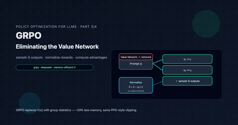
TL;DR: GRPO (Group Relative Policy Optimization) replaces PPO’s learned value function with a simple insight: sample outputs per prompt and use their normalized relative rewards as advantages. This eliminates ~33% of memory overhead while maintaining (or exceeding) PPO’s performance. The algorithm powers DeepSeekMath’s 51.7% MATH benchmark score and later became central to DeepSeek-R1’s remarkable reasoning capabilities.
Reading time: ~32 minutes
Prerequisites: Part 2: PPO for Language Models covers the clipped objective and GAE that GRPO builds upon.
The Memory Problem Revisited
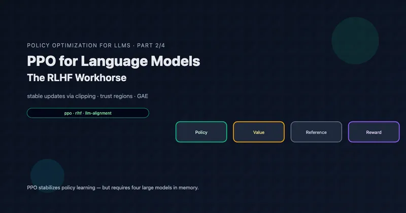
In Part 2, we saw PPO’s four-model architecture:
| Model | Purpose | Memory (7B) |
|---|---|---|
| Policy | Generate responses | ~28 GB |
| Reference | KL anchor | ~14 GB |
| Value | Advantage estimation | ~28 GB |
| Reward | Score responses | ~14 GB |
| Total | ~84 GB |
The value network accounts for one-third of memory, and it’s there for a single purpose: estimating advantages via GAE.
But what if we didn’t need to learn ? What if we could estimate advantages directly from samples?
This is GRPO’s insight: instead of learning “how good is this state?”, just sample multiple completions for the same prompt and compare them. The mean reward becomes your baseline. No neural network required.
Table of Contents
- The Core Insight: Group-Relative Advantages
- Mathematical Formulation
- Why This Works
- Outcome vs. Process Supervision
- Decoupled KL Regularization
- Iterative GRPO
- PyTorch Implementation
- DeepSeek-R1: GRPO at Scale
- A Unified View: GRPO, PPO, DPO, and RFT
- Limitations and When to Use Alternatives
- Key Takeaways
The Core Insight: Group-Relative Advantages
The Algorithm
For each prompt , GRPO:
- Sample a group of outputs from the current policy
- Score each output with the reward model:
- Normalize rewards using group statistics
- Use normalized rewards as advantages for all tokens in each output
The advantage for output is:
where are rewards for all outputs in the group.
That’s it. No learned value function. No GAE computation. Just sample, score, normalize.
Visual Comparison
Memory Savings
| Component | PPO | GRPO |
|---|---|---|
| Policy (training) | ~28 GB | ~28 GB |
| Reference (frozen) | ~14 GB | ~14 GB |
| Value (training) | ~28 GB | 0 GB |
| Reward (inference) | ~14 GB | ~14 GB |
| Total | ~84 GB | ~56 GB |
A 33% reduction in model memory. For large models, this often makes the difference between fitting on available hardware and needing more GPUs.
Key Insight: GRPO trades compute (sampling outputs per prompt) for memory (no value network). For LLMs where memory is the bottleneck, this is an excellent trade.
Mathematical Formulation
Let’s formalize GRPO precisely.
The GRPO Objective
GRPO maximizes:
The Per-Token Loss
Like PPO, GRPO uses the clipped surrogate objective:
where the importance ratio is:
The clipping mechanism is identical to PPO—what changes is how we compute .
Group-Relative Advantage Estimation
For outcome supervision (the standard case), all tokens in output share the same advantage:
where:
- is the reward for output
- are rewards for all outputs
Properties of Group-Relative Advantages
1. Zero-mean (approximately): Within each group, advantages sum to approximately zero:
This provides balanced training signal: reinforcing good outputs requires suppressing worse ones.
2. Unit variance: By dividing by std, advantages are normalized:
This makes gradients comparable across prompts with different reward scales.
3. Relative, not absolute: The advantage measures performance relative to the group, not absolute quality. An output with reward 0.5 could have positive advantage (if others scored 0.3) or negative (if others scored 0.7).
Why This Works
The group-relative approach succeeds for several reasons:
1. Natural Baseline
The mean reward estimates the expected reward under the current policy for this prompt:
With samples (as in DeepSeekMath), this estimate is reasonably accurate. This is exactly what we want from a baseline.
2. Matched to Reward Model Training
Reward models are typically trained on comparisons between outputs for the same prompt:
- “Output A is better than output B for prompt q”
GRPO’s group-relative advantages align with this comparative signal. We’re asking: “Among these outputs, which are better?“
3. Automatic Scale Normalization
Different prompts may have different “difficulty,” leading to different reward distributions:
- Easy prompt: All outputs score 0.8-0.9
- Hard prompt: All outputs score 0.2-0.4
Dividing by std normalizes these, preventing easy prompts from dominating gradients.
4. No Bootstrapping Bias
GAE uses estimates, introducing bias if the value function is inaccurate. GRPO uses only observed rewards—no bootstrapping, no bias from learned estimates.
5. Simplicity
The entire advantage computation is:
advantages = (rewards - rewards.mean()) / (rewards.std() + eps)
No recursive GAE computation, no value function forward passes, no TD errors.
Key Insight: The group mean is a Monte Carlo estimate of for this prompt. By sampling enough outputs, we get a good baseline without learning anything.
Outcome vs. Process Supervision
GRPO supports two supervision modes.
Outcome Supervision (Default)
A single reward at sequence end:
All tokens receive the same advantage—the normalized final reward.
Pros:
- Simple: Works with any output-level reward model
- Stable: Single reward signal, no step-level noise
Cons:
- Coarse credit assignment: Every token gets equal “blame” or “credit”
Process Supervision
Rewards at each reasoning step (e.g., separated by newlines):
Let be the token index at the end of step , and the total steps in output .
Step 1: Normalize per-step rewards
where contains all step rewards across all outputs in the group.
Step 2: Compute return-to-go
The advantage at token is the sum of normalized rewards from all subsequent steps.
Which to Choose?
| Situation | Recommendation |
|---|---|
| Standard RLHF | Outcome supervision |
| Multi-step reasoning (math, code) | Process supervision if PRM available |
| No process reward model | Outcome supervision |
| Training stability concerns | Outcome supervision |
DeepSeekMath experiments show process supervision slightly outperforms outcome supervision for math, but the difference is modest. Unless you have a high-quality Process Reward Model (PRM), outcome supervision is the simpler default.
Decoupled KL Regularization
GRPO handles KL penalty differently from standard PPO.
PPO: KL in the Reward
Standard PPO-RLHF adds KL to the per-token reward:
This KL penalty flows into GAE computation, coupling reward signal with regularization.
GRPO: KL in the Loss
GRPO adds KL directly to the loss, decoupled from advantages:
The Schulman KL Estimator
GRPO uses an unbiased KL estimator:
Properties:
- Non-negative: Always
- Zero at equality: Exactly 0 when
- Unbiased: Correct expectation under sampling
Why Decouple?
1. Cleaner advantage signal: Advantages reflect only task performance, not regularization.
2. Independent tuning: KL coefficient doesn’t interact with advantage normalization.
3. Simpler implementation: No need to track per-token KL during advantage computation.
Key Insight: Decoupling KL from rewards simplifies the algorithm. The policy gradient focuses on task performance; the KL term separately ensures we don’t drift too far from the reference.
Iterative GRPO
As training progresses, the reward model may become a poor discriminator for the improved policy’s outputs. Iterative GRPO addresses this.
The Staleness Problem
- Initially: Policy outputs vary in quality; reward model discriminates well
- After training: Policy consistently produces good outputs; reward model’s training distribution no longer matches
- Result: Degraded training signal
The Solution: Co-evolve Policy and Reward Model
Algorithm: Iterative GRPO

For iteration = 1, ..., I:

    ┌─────────────────────────────────────────────────────┐
    │ Phase 1: Reset Reference                            │
    └─────────────────────────────────────────────────────┘
    π_ref ← π_θ   (current policy becomes new reference)

    ┌─────────────────────────────────────────────────────┐
    │ Phase 2: Policy Training                            │
    └─────────────────────────────────────────────────────┘
    For step = 1, ..., M:
        Sample batch of prompts
        Sample G outputs per prompt from π_θ
        Compute rewards using r_φ
        Compute group-relative advantages
        Update π_θ using GRPO objective

    ┌─────────────────────────────────────────────────────┐
    │ Phase 3: Reward Model Update                        │
    └─────────────────────────────────────────────────────┘
    Generate comparison data from improved π_θ
    Continually train r_φ with:
        - 90% new data (from current policy)
        - 10% historical data (replay buffer)
Key Design Choices
Reference reset: Each iteration starts fresh, allowing larger cumulative policy drift while constraining per-iteration change.
Replay buffer: 10% historical data prevents the reward model from forgetting how to score earlier, easier outputs.
Single GRPO update: DeepSeekMath uses one gradient step per sample batch (), prioritizing fresh samples over reuse.
PyTorch Implementation
Here’s a complete, educational implementation of GRPO:
"""
Group Relative Policy Optimization (GRPO)
=========================================

Memory-efficient alternative to PPO that eliminates the value network
by computing advantages from groups of sampled outputs.

Reference: DeepSeekMath (Shao et al., 2024)
"""

import torch
import torch.nn.functional as F
from torch import Tensor
from dataclasses import dataclass
from typing import Tuple, List


@dataclass
class GRPOConfig:
    """GRPO hyperparameters."""

    # Core settings
    group_size: int = 64           # G: outputs per prompt
    clip_epsilon: float = 0.2      # ε: PPO clipping
    kl_coef: float = 0.04          # β: KL penalty coefficient

    # Generation
    max_length: int = 1024
    temperature: float = 1.0

    # Training
    learning_rate: float = 1e-6
    max_grad_norm: float = 1.0

    # Numerical stability
    eps: float = 1e-8


def compute_group_advantages(rewards: Tensor, eps: float = 1e-8) -> Tensor:
    """
    Compute group-relative advantages.

    This is GRPO's key innovation: use group statistics
    instead of a learned value function.

    Args:
        rewards: [G] rewards for each output in the group
        eps: Small constant for numerical stability

    Returns:
        advantages: [G] normalized advantages
    """
    mean_r = rewards.mean()
    std_r = rewards.std() + eps
    advantages = (rewards - mean_r) / std_r
    return advantages


def compute_schulman_kl(
    policy_log_probs: Tensor,
    reference_log_probs: Tensor,
) -> Tensor:
    """
    Compute Schulman's unbiased KL estimator.

    D_KL = π_ref/π_θ - log(π_ref/π_θ) - 1

    This estimator is:
    - Non-negative (always >= 0)
    - Unbiased (correct expectation)
    - Zero when π_θ = π_ref

    Args:
        policy_log_probs: [batch, seq_len] from π_θ
        reference_log_probs: [batch, seq_len] from π_ref

    Returns:
        kl: [batch, seq_len] per-token KL
    """
    log_ratio = reference_log_probs - policy_log_probs  # log(π_ref/π_θ)
    kl = torch.exp(log_ratio) - log_ratio - 1
    return kl


def compute_grpo_loss(
    policy_log_probs: Tensor,
    old_log_probs: Tensor,
    reference_log_probs: Tensor,
    advantages: Tensor,
    response_mask: Tensor,
    clip_epsilon: float = 0.2,
    kl_coef: float = 0.04,
) -> Tuple[Tensor, dict]:
    """
    Compute GRPO loss with clipping and KL penalty.

    Args:
        policy_log_probs: [G, seq_len] current policy
        old_log_probs: [G, seq_len] policy at sampling time
        reference_log_probs: [G, seq_len] reference policy
        advantages: [G] per-output advantages (will broadcast)
        response_mask: [G, seq_len] valid token mask
        clip_epsilon: PPO clipping parameter
        kl_coef: KL penalty coefficient

    Returns:
        loss: Scalar loss to minimize
        metrics: Dictionary of training metrics
    """
    G, seq_len = policy_log_probs.shape

    # =========================================
    # 1. Importance ratio: ρ = π_θ / π_old
    # =========================================
    log_ratio = policy_log_probs - old_log_probs
    ratio = torch.exp(log_ratio)  # [G, seq_len]

    # =========================================
    # 2. Expand advantages to token level
    # =========================================
    # [G] -> [G, seq_len]
    token_advantages = advantages.unsqueeze(1).expand(-1, seq_len)

    # =========================================
    # 3. PPO clipped objective
    # =========================================
    clipped_ratio = torch.clamp(ratio, 1 - clip_epsilon, 1 + clip_epsilon)

    policy_loss_1 = ratio * token_advantages
    policy_loss_2 = clipped_ratio * token_advantages
    policy_loss = torch.min(policy_loss_1, policy_loss_2)

    # =========================================
    # 4. KL penalty (decoupled from reward)
    # =========================================
    kl_penalty = compute_schulman_kl(policy_log_probs, reference_log_probs)

    # =========================================
    # 5. Combine losses
    # =========================================
    # Maximize policy objective, minimize KL
    token_loss = -policy_loss + kl_coef * kl_penalty

    # Mask and average
    masked_loss = token_loss * response_mask
    per_output_loss = masked_loss.sum(dim=1) / response_mask.sum(dim=1).clamp(min=1)
    loss = per_output_loss.mean()

    # =========================================
    # 6. Metrics
    # =========================================
    with torch.no_grad():
        clip_fraction = ((ratio - 1).abs() > clip_epsilon).float()
        clip_fraction = (clip_fraction * response_mask).sum() / response_mask.sum()

        mean_kl = (kl_penalty * response_mask).sum() / response_mask.sum()

    metrics = {
        "loss": loss.item(),
        "clip_fraction": clip_fraction.item(),
        "mean_kl": mean_kl.item(),
        "mean_advantage": advantages.mean().item(),
        "advantage_std": advantages.std().item(),
    }

    return loss, metrics


class GRPOTrainer:
    """
    GRPO trainer for LLM fine-tuning.

    Unlike PPO, requires only THREE models (no value network):
    - policy_model: The LLM being trained
    - reference_model: Frozen copy for KL penalty
    - reward_model: Scores complete responses

    Memory savings: ~33% compared to PPO
    """

    def __init__(
        self,
        policy_model: torch.nn.Module,
        reference_model: torch.nn.Module,
        reward_model,  # Can be a function or model
        tokenizer,
        config: GRPOConfig,
    ):
        self.policy = policy_model
        self.reference = reference_model
        self.reward_fn = reward_model
        self.tokenizer = tokenizer
        self.config = config

        # Freeze reference model
        for param in self.reference.parameters():
            param.requires_grad = False

        # Single optimizer (no value network!)
        self.optimizer = torch.optim.AdamW(
            self.policy.parameters(),
            lr=config.learning_rate,
            betas=(0.9, 0.95),
            weight_decay=0.1
        )

    @torch.no_grad()
    def sample_group(
        self,
        prompt_ids: Tensor,
        attention_mask: Tensor,
    ) -> Tuple[Tensor, Tensor]:
        """
        Sample G outputs for a single prompt.

        Args:
            prompt_ids: [1, prompt_len] token ids
            attention_mask: [1, prompt_len]

        Returns:
            output_ids: [G, total_len] generated sequences
            output_masks: [G, total_len] attention masks
        """
        G = self.config.group_size
        device = prompt_ids.device

        # Expand prompt for batch generation
        prompt_ids = prompt_ids.expand(G, -1)
        attention_mask = attention_mask.expand(G, -1)

        # Sample from policy
        self.policy.eval()
        outputs = self.policy.generate(
            input_ids=prompt_ids,
            attention_mask=attention_mask,
            max_new_tokens=self.config.max_length,
            do_sample=True,
            temperature=self.config.temperature,
            pad_token_id=self.tokenizer.pad_token_id,
            return_dict_in_generate=True,
        )

        output_ids = outputs.sequences
        output_masks = (output_ids != self.tokenizer.pad_token_id).long()

        return output_ids, output_masks

    @torch.no_grad()
    def compute_rewards(
        self,
        prompt_text: str,
        output_ids: Tensor,
        prompt_len: int,
    ) -> Tensor:
        """
        Compute rewards for each output in the group.

        Args:
            prompt_text: The original prompt string
            output_ids: [G, total_len] generated sequences
            prompt_len: Length of prompt in tokens

        Returns:
            rewards: [G] scalar reward per output
        """
        G = output_ids.shape[0]
        rewards = []

        for i in range(G):
            # Extract response tokens
            response_ids = output_ids[i, prompt_len:]
            response_text = self.tokenizer.decode(
                response_ids, skip_special_tokens=True
            )

            # Score with reward model
            reward = self.reward_fn(prompt_text, response_text)
            rewards.append(reward)

        return torch.tensor(rewards, device=output_ids.device)

    def compute_log_probs(
        self,
        model: torch.nn.Module,
        input_ids: Tensor,
        attention_mask: Tensor,
        response_start_idx: int,
    ) -> Tensor:
        """
        Compute per-token log probabilities for response tokens.

        Args:
            model: Language model
            input_ids: [batch, seq_len] full sequences
            attention_mask: [batch, seq_len]
            response_start_idx: Where response tokens begin

        Returns:
            log_probs: [batch, response_len] per-token log probs
        """
        outputs = model(
            input_ids=input_ids,
            attention_mask=attention_mask,
            return_dict=True,
        )
        logits = outputs.logits  # [batch, seq_len, vocab]

        # Shift for next-token prediction
        shift_logits = logits[:, :-1, :]
        shift_labels = input_ids[:, 1:]

        # Log probabilities
        log_probs = F.log_softmax(shift_logits, dim=-1)

        # Gather log probs for actual tokens
        token_log_probs = log_probs.gather(
            dim=-1,
            index=shift_labels.unsqueeze(-1)
        ).squeeze(-1)

        # Extract response tokens only
        response_log_probs = token_log_probs[:, response_start_idx - 1:]

        return response_log_probs

    def train_step(
        self,
        prompt_text: str,
        prompt_ids: Tensor,
        attention_mask: Tensor,
    ) -> dict:
        """
        Single GRPO training step.

        Args:
            prompt_text: Original prompt string
            prompt_ids: [1, prompt_len] tokenized prompt
            attention_mask: [1, prompt_len]

        Returns:
            metrics: Training metrics dictionary
        """
        prompt_len = prompt_ids.shape[1]
        device = prompt_ids.device

        # =============================================
        # Step 1: Sample group of outputs
        # =============================================
        output_ids, output_masks = self.sample_group(prompt_ids, attention_mask)
        G = output_ids.shape[0]

        # =============================================
        # Step 2: Compute rewards
        # =============================================
        rewards = self.compute_rewards(prompt_text, output_ids, prompt_len)

        # =============================================
        # Step 3: Compute group-relative advantages
        # =============================================
        advantages = compute_group_advantages(rewards, self.config.eps)

        # =============================================
        # Step 4: Get log probs (old = current pre-update)
        # =============================================
        with torch.no_grad():
            old_log_probs = self.compute_log_probs(
                self.policy, output_ids, output_masks, prompt_len
            )
            reference_log_probs = self.compute_log_probs(
                self.reference, output_ids, output_masks, prompt_len
            )

        # =============================================
        # Step 5: Policy gradient update
        # =============================================
        self.policy.train()

        policy_log_probs = self.compute_log_probs(
            self.policy, output_ids, output_masks, prompt_len
        )

        # Response mask
        response_mask = output_masks[:, prompt_len:]

        loss, metrics = compute_grpo_loss(
            policy_log_probs,
            old_log_probs,
            reference_log_probs,
            advantages,
            response_mask,
            self.config.clip_epsilon,
            self.config.kl_coef,
        )

        self.optimizer.zero_grad()
        loss.backward()
        torch.nn.utils.clip_grad_norm_(
            self.policy.parameters(),
            self.config.max_grad_norm
        )
        self.optimizer.step()

        # Add reward metrics
        metrics["mean_reward"] = rewards.mean().item()
        metrics["reward_std"] = rewards.std().item()

        return metrics
Implementation Notes
Group size selection: DeepSeekMath uses . Larger groups give more stable advantage estimates. Reasonable range: 16-128.
Single update per sample: The implementation does one gradient step per sampled batch. Multiple steps would require re-computing advantages as the policy changes.
KL coefficient: Start with . Lower values allow more divergence; higher values constrain updates.
DeepSeek-R1: GRPO at Scale
In January 2025, DeepSeek released DeepSeek-R1, a reasoning model matching OpenAI’s o1 on many benchmarks. GRPO is central to its training.
R1’s Training Pipeline
Why GRPO for R1?
1. Long reasoning traces: R1 produces outputs with thousands of tokens. A value network would need to predict final reward from any point in this long sequence—extremely difficult.
2. Verifiable rewards: For math and code, rewards are rule-based (correct/incorrect). No reward model uncertainty.
3. Memory efficiency: At R1’s scale, GRPO’s memory savings are crucial.
4. Training stability: Simpler architecture means fewer things can go wrong.
The “Aha Moment” Phenomenon
The R1 paper describes emergent behavior during GRPO training: the model spontaneously developed “aha moment” patterns—places where it reconsiders and corrects earlier reasoning mistakes.
Example reasoning trace:
"Let me solve this step by step...
 First, I'll set up the equation: 2x + 5 = 13
 Subtracting 5: 2x = 8
 Wait, let me verify that. 13 - 5 = 8. Yes, correct.
 Dividing by 2: x = 4

 Let me check: 2(4) + 5 = 8 + 5 = 13 ✓

 The answer is x = 4."
This self-correction emerged without explicit supervision—GRPO’s optimization pressure (combined with correctness rewards) naturally discovered it.
R1-Zero: Pure RL Without SFT
DeepSeek also released R1-Zero, trained with GRPO directly from the base model without any SFT stage. Remarkably, it still develops coherent reasoning, though with some readability issues that the full R1 pipeline addresses.
This demonstrates GRPO’s power: given only a correctness signal, the algorithm can induce sophisticated reasoning behavior.
Key Insight: GRPO’s simplicity makes it stable enough for extreme-scale training. DeepSeek-R1 shows that you can train world-class reasoning models without the complexity of PPO’s value network.
A Unified View: GRPO, PPO, DPO, and RFT
The DeepSeekMath paper provides a unified framework for understanding different alignment methods.
The General Policy Gradient
All methods can be viewed through:
Methods differ in:
- Data source : Where do samples come from?
- Gradient coefficient : How are outputs weighted?
Method Comparison
| Method | Data Source | Coefficient | Online? |
|---|---|---|---|
| SFT | Human demos | (uniform) | ❌ |
| RFT | Filtered policy samples | (filtered) | ❌ |
| DPO | Preference pairs | ❌ | |
| Online RFT | Current policy | (filtered) | ✅ |
| PPO | Current policy | (GAE) | ✅ |
| GRPO | Current policy | (group-normalized) | ✅ |
Key Insights
Online vs. Offline: GRPO, PPO, and Online RFT sample from the current policy and can adapt. DPO and RFT use fixed datasets.
Weighted vs. Filtered: RFT keeps only correct outputs (binary filter). GRPO keeps all outputs but weights by normalized reward (continuous weighting).
Advantage estimation: PPO learns ; GRPO uses group statistics; DPO implicitly computes advantages through preferences.
Limitations and When to Use Alternatives
GRPO Limitations
1. Sampling cost: outputs per prompt (typically 64). More compute than PPO’s single sample.
2. Advantage variance: With small groups, the mean is a noisy baseline. Need for stability.
3. Uniform token credit: All tokens get the same advantage. No fine-grained credit assignment without process supervision.
4. Reward model dependency: Like all RL methods, susceptible to reward hacking if the reward model has exploits.
5. No value function benefits: Can’t use value-guided search or intrinsic motivation bonuses.
When to Use Each Method
| Situation | Recommendation |
|---|---|
| Memory-constrained | ✅ GRPO |
| Compute-constrained | Consider PPO |
| Outcome rewards only | ✅ GRPO |
| Dense per-step rewards | Consider PPO (GAE) |
| Offline preferences only | Use DPO |
| No reward model | Use DPO or RFT |
| Value-guided search needed | Use PPO |
| Multi-reward training | Use GDPO (Part 4) |
Key Takeaways
The Core Innovation
Sample multiple outputs, normalize rewards, use as advantages. No value network.
Memory Savings
- Eliminates ~28GB value network (for 7B model)
- 33% reduction in model memory
- Often the difference between 1 GPU and multiple
Design Choices
- Group size: for stability
- Clip epsilon: (standard PPO)
- KL coefficient:
- Decoupled KL: In loss, not reward
When GRPO Excels
- Memory-constrained training
- Outcome-based rewards
- Long generations (where value prediction is hard)
- Verifiable rewards (math, code)
DeepSeek-R1 Connection
GRPO powers R1’s remarkable reasoning through:
- Rule-based correctness rewards
- Emergent self-correction (“aha moments”)
- Stable training at scale
What’s Next
In Part 4: GDPO, we’ll see what happens when GRPO meets multi-reward settings:
- Why combined reward normalization causes “advantage collapse”
- GDPO’s solution: decouple normalization per reward
- Production patterns for tool calling, math, and coding
Further Reading
Original Papers:
- DeepSeekMath: Pushing the Limits of Mathematical Reasoning (Shao et al., 2024)
- DeepSeek-R1: Incentivizing Reasoning Capability in LLMs via Reinforcement Learning (DeepSeek-AI, 2025)
Related Work:
- Proximal Policy Optimization (Schulman et al., 2017)
- Direct Preference Optimization (Rafailov et al., 2023)
Implementations:
Article series
Policy Optimization for LLMs: From Fundamentals to Production
- Part 1 Reinforcement Learning Foundations for LLM Alignment
- Part 2 PPO for Language Models: The RLHF Workhorse
- Part 3 GRPO: Eliminating the Value Network
- Part 4 GDPO: Multi-Reward RL Done Right